# Import
import pandas as pd
import numpy as np
from sklearn.preprocessing import LabelEncoder
from warnings import simplefilter
from sklearn.exceptions import ConvergenceWarning
simplefilter("ignore", category=ConvergenceWarning) # avoid warning
from sklearn.linear_model import LogisticRegression
from sklearn.ensemble import RandomForestClassifier
from sklearn.svm import SVC
from sklearn.preprocessing import StandardScaler
from sklearn.linear_model import LogisticRegression
from matplotlib import pyplot as plt
from sklearn.model_selection import cross_val_score
from sklearn.tree import DecisionTreeClassifier
from sklearn.tree import DecisionTreeClassifier, plot_tree
from sklearn.model_selection import GridSearchCV
from matplotlib.patches import Patch
from itertools import combinations
import seaborn as snsIntroduction
In this blog post, I will work through a complete example of the standard machine learning workflow by classifying three penguine species: chinstrap, gentoo, and adelie. My primary goal is to determine the smallest number of measurements necessary to confidently determine the species of a penguin. I will first inspect the dataset and prepare the dataset by dropping columns that are not needed and converting binary variables into dummy variables that are machine-readable. Then, I will conduct some data exploration which includes 1) grouping the penguins by sex and inspect their body mass, and 2) using the pair plot to eye-ball the associative relationship between each features. Next, I will use four models (logistic regression, decision tree, support vector machine, and random forest) to determine what are the best features for classification. All of the models ended up choosing the same features. Then I will train and test all the models, assessing their performance by accuracy on the test dataset. Finally, I will plot the decision regions to visualize how each model classifies the penguins in both training and testing datasets. The conclusion I got is that the logistic regression model works the best.
Data Inspection
I firstly inspect the training data by importing it as a data frame. The dataset is called the Palmer Penguins data, collected by Dr. Kristen Gorman and the Palmer Station, Antarctica LTER, a member of the Long Term Ecological Research Network based on the information given to me (https://middlebury-csci-0451.github.io/CSCI-0451/assignments/blog-posts/blog-post-penguins.html).
train_url = "https://raw.githubusercontent.com/middlebury-csci-0451/CSCI-0451/main/data/palmer-penguins/train.csv"
train = pd.read_csv(train_url)train.head()| studyName | Sample Number | Species | Region | Island | Stage | Individual ID | Clutch Completion | Date Egg | Culmen Length (mm) | Culmen Depth (mm) | Flipper Length (mm) | Body Mass (g) | Sex | Delta 15 N (o/oo) | Delta 13 C (o/oo) | Comments | |
|---|---|---|---|---|---|---|---|---|---|---|---|---|---|---|---|---|---|
| 0 | PAL0708 | 27 | Gentoo penguin (Pygoscelis papua) | Anvers | Biscoe | Adult, 1 Egg Stage | N46A1 | Yes | 11/29/07 | 44.5 | 14.3 | 216.0 | 4100.0 | NaN | 7.96621 | -25.69327 | NaN |
| 1 | PAL0708 | 22 | Gentoo penguin (Pygoscelis papua) | Anvers | Biscoe | Adult, 1 Egg Stage | N41A2 | Yes | 11/27/07 | 45.1 | 14.5 | 215.0 | 5000.0 | FEMALE | 7.63220 | -25.46569 | NaN |
| 2 | PAL0910 | 124 | Adelie Penguin (Pygoscelis adeliae) | Anvers | Torgersen | Adult, 1 Egg Stage | N67A2 | Yes | 11/16/09 | 41.4 | 18.5 | 202.0 | 3875.0 | MALE | 9.59462 | -25.42621 | NaN |
| 3 | PAL0910 | 146 | Adelie Penguin (Pygoscelis adeliae) | Anvers | Dream | Adult, 1 Egg Stage | N82A2 | Yes | 11/16/09 | 39.0 | 18.7 | 185.0 | 3650.0 | MALE | 9.22033 | -26.03442 | NaN |
| 4 | PAL0708 | 24 | Chinstrap penguin (Pygoscelis antarctica) | Anvers | Dream | Adult, 1 Egg Stage | N85A2 | No | 11/28/07 | 50.6 | 19.4 | 193.0 | 3800.0 | MALE | 9.28153 | -24.97134 | NaN |
Data Prep
I then prepare the data by dropping the columns of “studyName”, “Sample Number”, “Individual ID”, “Date Egg”, “Comments”, “Region” to keep the data frame relatively small for facilitating further analysis. I also transform binary variables including the island names, their adult stage, clutch completion, and sex into dummy variables.
le = LabelEncoder()
le.fit(train["Species"])

def prepare_data(df):
  df = df.drop(["studyName", "Sample Number", "Individual ID", "Date Egg", "Comments", "Region"], axis = 1)
  df = df[df["Sex"] != "."]
  df = df.dropna()
  y = le.transform(df["Species"])
  df = df.drop(["Species"], axis = 1)
  df = pd.get_dummies(df)
  return df, y

X_train, y_train = prepare_data(train)X_train.head()| Culmen Length (mm) | Culmen Depth (mm) | Flipper Length (mm) | Body Mass (g) | Delta 15 N (o/oo) | Delta 13 C (o/oo) | Island_Biscoe | Island_Dream | Island_Torgersen | Stage_Adult, 1 Egg Stage | Clutch Completion_No | Clutch Completion_Yes | Sex_FEMALE | Sex_MALE | |
|---|---|---|---|---|---|---|---|---|---|---|---|---|---|---|
| 1 | 45.1 | 14.5 | 215.0 | 5000.0 | 7.63220 | -25.46569 | 1 | 0 | 0 | 1 | 0 | 1 | 1 | 0 |
| 2 | 41.4 | 18.5 | 202.0 | 3875.0 | 9.59462 | -25.42621 | 0 | 0 | 1 | 1 | 0 | 1 | 0 | 1 |
| 3 | 39.0 | 18.7 | 185.0 | 3650.0 | 9.22033 | -26.03442 | 0 | 1 | 0 | 1 | 0 | 1 | 0 | 1 |
| 4 | 50.6 | 19.4 | 193.0 | 3800.0 | 9.28153 | -24.97134 | 0 | 1 | 0 | 1 | 1 | 0 | 0 | 1 |
| 5 | 33.1 | 16.1 | 178.0 | 2900.0 | 9.04218 | -26.15775 | 0 | 1 | 0 | 1 | 0 | 1 | 1 | 0 |
y_trainarray([2, 0, 0, 1, 0, 0, 0, 2, 0, 2, 0, 0, 1, 1, 1, 2, 1, 2, 2, 0, 0, 1,
2, 2, 0, 2, 0, 1, 1, 0, 0, 0, 2, 0, 2, 0, 0, 0, 2, 0, 0, 0, 0, 0,
1, 0, 2, 2, 2, 1, 1, 1, 2, 2, 2, 0, 2, 0, 2, 2, 2, 0, 2, 1, 0, 0,
2, 0, 2, 2, 0, 2, 0, 0, 2, 1, 1, 2, 2, 0, 1, 2, 2, 2, 1, 0, 1, 0,
0, 0, 0, 1, 2, 0, 2, 0, 0, 2, 0, 2, 2, 0, 0, 1, 0, 2, 0, 2, 0, 2,
0, 0, 2, 2, 0, 2, 0, 2, 0, 2, 0, 2, 0, 2, 2, 0, 2, 0, 2, 0, 2, 2,
0, 2, 2, 0, 1, 2, 1, 2, 0, 0, 0, 2, 0, 0, 1, 1, 0, 2, 1, 2, 2, 2,
2, 0, 2, 0, 0, 0, 0, 1, 0, 0, 2, 2, 0, 2, 0, 1, 0, 1, 2, 1, 1, 1,
2, 0, 1, 0, 0, 1, 0, 0, 2, 0, 1, 1, 0, 1, 1, 0, 0, 1, 0, 2, 1, 2,
0, 1, 2, 0, 2, 2, 1, 1, 0, 2, 0, 0, 2, 1, 0, 2, 2, 1, 1, 2, 2, 2,
0, 2, 2, 2, 2, 0, 0, 1, 2, 1, 2, 2, 1, 2, 0, 1, 0, 0, 0, 0, 1, 2,
0, 1, 1, 0, 2, 0, 1, 1, 1, 0, 2, 0, 2, 2])Data Exploration
In the following table, I group the data by sex and calculate the mean body mass for each sex. We can see from the result that the mean body mass of the male penguins is substantially higher than the mean body mass of the female penguins.
X_train.groupby(['Sex_MALE'])[['Body Mass (g)']].aggregate([np.mean,len ]).round(2)| Body Mass (g) | ||
|---|---|---|
| mean | len | |
| Sex_MALE | ||
| 0 | 3823.21 | 126 |
| 1 | 4613.08 | 130 |
In the subsequent pair chart, we inspect the correlation between each pair of features. We can see that the culmen length, the culmen depth, the flipper length, and the body mass are in general positively correlated with each other. It also seems like if we were to differentiate the species, Delta 15 N would be a good measurement because the means of the three clusters are more distinctly separated compared to that separation in other features. However, partially due to my misunderstanding of the instruction and limited time, I have removed the Delta 15 N previously to keep the training and testing process simple. We, thus, did not have a chance to see if this feature would be selected by the machine learning algorithms. Nevertheless, it is a good practice for future studies to draw the pair plot and inspect the relationships between features to determine which features to be kept or removed.
sns.set_theme(style="ticks")
sns.pairplot(train, hue="Species")
<seaborn.axisgrid.PairGrid at 0x7f7f9fd9da00>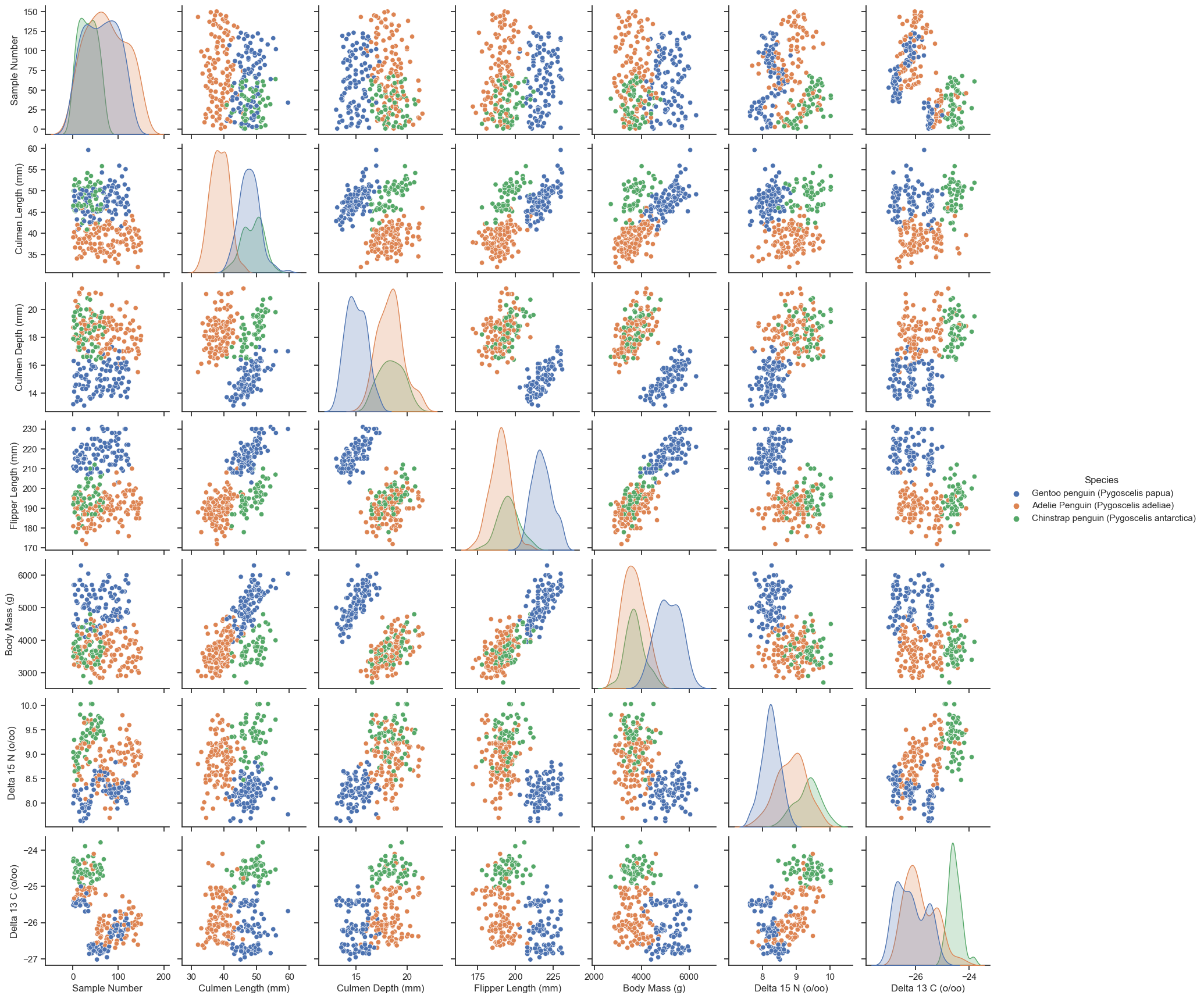
Choosing Features
In the following chunk of code, we loop through three models (logistic regression, support vector machine, and random forest) as well as the groups of features to determine what are the best three features (2 quantitative and 1 qualitative) to determine the species. The skeleton of the code is based on the blog instruction (https://middlebury-csci-0451.github.io/CSCI-0451/assignments/blog-posts/blog-post-penguins.html#your-challenge).
# Scale the model to prevent warnings
scaler = StandardScaler()
X_train_scaled = scaler.fit_transform(X_train)


# Search for the best columns witht the largest cross validation score
all_qual_cols = ["Clutch Completion", "Sex", "Island", "Stage"]
all_quant_cols = ['Culmen Length (mm)', 'Culmen Depth (mm)', 'Flipper Length (mm)', 'Body Mass (g)', 'Delta 15 N (o/oo)', 'Delta 13 C (o/oo)']

# Create a dictionary to store the models of interest
models = {
    "Logistic Regression": LogisticRegression(),
    "SVC": SVC(gamma = 0.01),
    "Random Forest": RandomForestClassifier()
}

# Initiate an empty array for the best cols, the score, and the best model
best_cols = None
best_score = 0
best_model = None

# Main loop to iterate through the feature groups
for model_name, model in models.items():
    print(f"Evaluating {model_name}...")
    for qual in all_qual_cols:
        qual_cols = [col for col in X_train.columns if qual in col]
        for pair in combinations(all_quant_cols, 2):
            cols =  list(pair) + qual_cols
            # print(cols)
            X_subset = X_train[cols]
            scores = cross_val_score(model, X_subset, y_train, cv=5) # You can modify the cv parameter as needed
            mean_score = scores.mean()
            if mean_score > best_score:
                best_cols = cols
                best_score = mean_score
                best_model = model_name

    print(f"The best score for {model_name} was {best_score} and the best columns were {best_cols}")

print(f"The best model was {best_model} with a score of {best_score} and the best columns were {best_cols}")
Evaluating Logistic Regression...
The best score for Logistic Regression was 0.996078431372549 and the best columns were ['Culmen Length (mm)', 'Culmen Depth (mm)', 'Island_Biscoe', 'Island_Dream', 'Island_Torgersen']
Evaluating SVC...
The best score for SVC was 0.996078431372549 and the best columns were ['Culmen Length (mm)', 'Culmen Depth (mm)', 'Island_Biscoe', 'Island_Dream', 'Island_Torgersen']
Evaluating Random Forest...
The best score for Random Forest was 0.996078431372549 and the best columns were ['Culmen Length (mm)', 'Culmen Depth (mm)', 'Island_Biscoe', 'Island_Dream', 'Island_Torgersen']
The best model was Logistic Regression with a score of 0.996078431372549 and the best columns were ['Culmen Length (mm)', 'Culmen Depth (mm)', 'Island_Biscoe', 'Island_Dream', 'Island_Torgersen']Our results showed that all models chose the same set of features, showing a strong evidence that these features are good choices for our classification. The scores across models were approximately the same.
Model Choices
To train the model, I firstly use logistic regression based on the instruction. Additionally, I also explore other models including decision tree, random forest, and SVC.
Logistic Regression
# Train/Fit & Calculate training score
LR = LogisticRegression()
LR.fit(X_train[best_cols], y_train)
LR_train_score = LR.score(X_train[best_cols], y_train)
print(f"{LR_train_score=}")LR_train_score=1.0Other Models
Decision Tree
# Use cross validation to find the best depth and plug back to the "Choosing Features" chunk
np.random.seed(12345)

fig, ax = plt.subplots(1)

for d in range(2, 5):
    T = DecisionTreeClassifier(max_depth = d)
    m = cross_val_score(T, X_train[cols], y_train, cv = 10).mean()
    ax.scatter(d, m, color = "black")
    # ax.scatter(d, T.score(X_test, y_test), color = "firebrick")

labs = ax.set(xlabel = "Complexity (depth)", ylabel = "Performance (score)")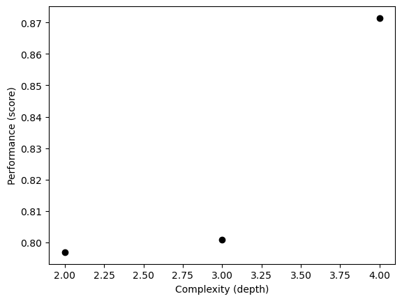
# Train/Fit & Calculate training score
DTC = DecisionTreeClassifier(max_depth = 3)
DTC.fit(X_train[best_cols], y_train)
DTC_train_score = DTC.score(X_train[best_cols], y_train)
print(f"{DTC_train_score=}")

# Show the decision tree plot
plt.figure(figsize=(12,12))
p = plot_tree(DTC, feature_names = best_cols, filled = True, class_names = species, fontsize=8)
plt.show()
DTC_train_score=0.9921875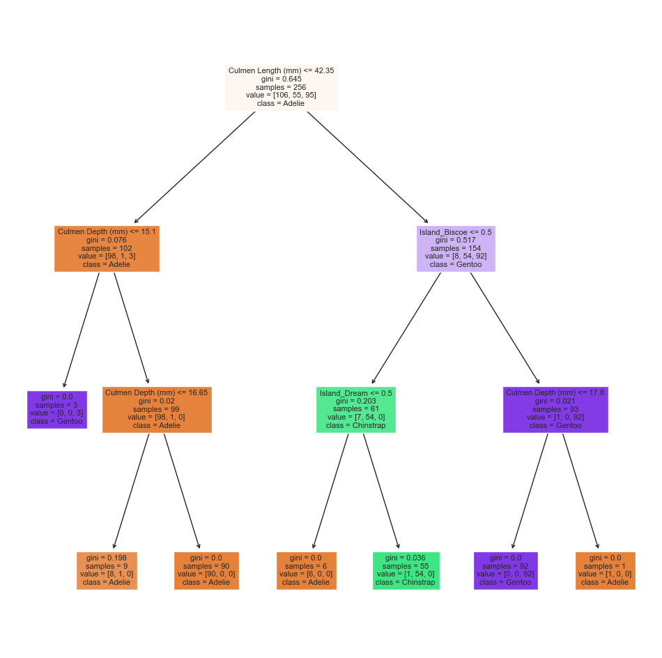
Random Forest
# Train/Fit & Calculate training score
rf = RandomForestClassifier()
rf.fit(X_train[best_cols], y_train)
rf_train_score = rf.score(X_train[best_cols], y_train)
print(f"{rf_train_score=}")rf_train_score=1.0SVC
# Use grid search to find the best gamma and plug back to the "Choosing Features" chunk
param_grid = {'gamma': np.logspace(-5, 5, num=11)}

svc = SVC()
grid_search = GridSearchCV(svc, param_grid, cv=5)
grid_search.fit(X_train, y_train)

print("Best gamma:", grid_search.best_params_['gamma'])
print("Best score:", grid_search.best_score_)
Best gamma: 0.01
Best score: 0.7730769230769232This gamma value is calculatef first and then used when seleting the features.
# Train/Fit & Calculate training score
svc_best = SVC(gamma = 0.01)
svc_best.fit(X_train[best_cols], y_train)
svc_train_score = svc_best.score(X_train[best_cols], y_train)
print(f"{svc_train_score=}")svc_train_score=0.98046875Our training results showed that logistic regression, decision tree, and random forest all have an accuracy of 100%, and SVC obtained a not-so-bad 98%.
Testing
# Get the test data
test_url = "https://raw.githubusercontent.com/middlebury-csci-0451/CSCI-0451/main/data/palmer-penguins/test.csv"
test = pd.read_csv(test_url)

X_test, y_test = prepare_data(test)

# LR
LR.fit(X_train[best_cols], y_train)
LR_score = LR.score(X_test[best_cols], y_test)
print("LR test score:", LR_score)

# Decision Tree
DTC.fit(X_train[best_cols], y_train)
DTC_score = DTC.score(X_test[best_cols], y_test)
print("Decision Tree test score:", DTC_score)

# Random Forest
rf = RandomForestClassifier()
rf.fit(X_train[best_cols], y_train)
rf_score = rf.score(X_test[best_cols], y_test)
print("Random Forest test score:", rf_score)

# SVC
svc_best = SVC(gamma=0.01)
svc_best.fit(X_train[best_cols], y_train)
svc_score = svc_best.score(X_test[best_cols], y_test)
print("SVC test score:", svc_score)
LR test score: 1.0
Decision Tree test score: 0.9852941176470589
Random Forest test score: 0.9852941176470589
SVC test score: 0.9264705882352942Our test results showed that LR seemed to be the best model with an accuracy of 100%, following it were the decision tree and random forest with the same accuracy of 98.5%, and the last one was SVC with a score of 92.6%, which is quite consistent with our training results.
Plotting Decision Regions
In this section, we plot the decision regions to visualize the peformance of classification for all of the models in both training and testing.
# The skeleton of the code is based on the blog instruction (https://middlebury-csci-0451.github.io/CSCI-0451/assignments/blog-posts/blog-post-penguins.html#your-challenge).
def plot_regions(model, X, y, model_name):

    x0 = X[X.columns[0]]
    x1 = X[X.columns[1]]
    qual_features = X.columns[2:]

    fig, axarr = plt.subplots(1, len(qual_features), figsize = (7, 3))

    # create a grid
    grid_x = np.linspace(x0.min(),x0.max(),501)
    grid_y = np.linspace(x1.min(),x1.max(),501)
    xx, yy = np.meshgrid(grid_x, grid_y)

    # add the title
    fig.suptitle(model_name + " Decision Boundaries", fontsize=14)

    XX = xx.ravel()
    YY = yy.ravel()

    for i in range(len(qual_features)):
      XY = pd.DataFrame({
          X.columns[0] : XX,
          X.columns[1] : YY
      })

      for j in qual_features:
        XY[j] = 0

      XY[qual_features[i]] = 1

      p = model.predict(XY)
      p = p.reshape(xx.shape)


      # use contour plot to visualize the predictions
      axarr[i].contourf(xx, yy, p, cmap = "jet", alpha = 0.2, vmin = 0, vmax = 2)

      ix = X[qual_features[i]] == 1
      # plot the data
      axarr[i].scatter(x0[ix], x1[ix], c = y[ix], cmap = "jet", vmin = 0, vmax = 2)

      axarr[i].set(xlabel = X.columns[0],
            ylabel  = X.columns[1])

      patches = []
      for color, spec in zip(["red", "green", "blue"], ["Adelie", "Chinstrap", "Gentoo"]):
        patches.append(Patch(color = color, label = spec))

      plt.legend(title = "Species", handles = patches, loc = "best")

      plt.tight_layout()
Decision Boundaries for Training Data
plot_regions(LR, X_train[best_cols], y_train, model_name = "LR")
plot_regions(DTC, X_train[best_cols], y_train, model_name = "DTC")
plot_regions(rf, X_train[best_cols], y_train, model_name = "Random Forest")
plot_regions(svc_best, X_train[best_cols], y_train, model_name = "Support Vector Machine")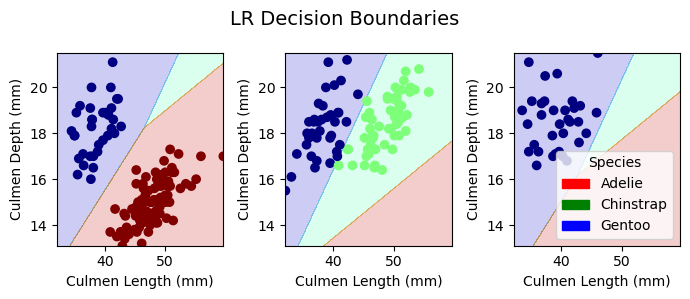
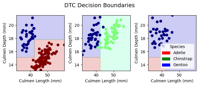
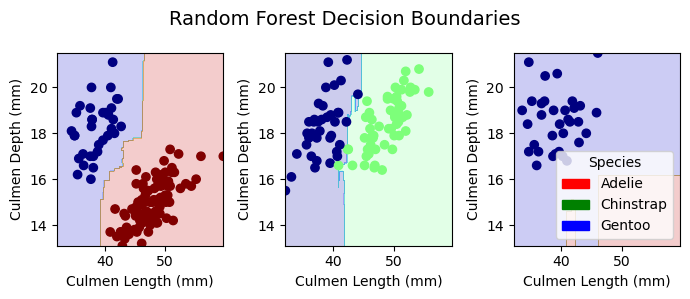
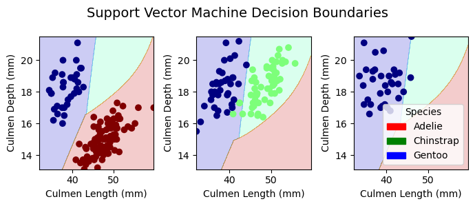
Decision Boundaries for Testing Data
plot_regions(LR, X_test[best_cols], y_test, model_name = "LR")
plot_regions(DTC, X_test[best_cols], y_test, model_name = "DTC")
plot_regions(rf, X_test[best_cols], y_test, model_name = "Random Forest")
plot_regions(svc_best, X_test[best_cols], y_test, model_name = "Support Vector Machine")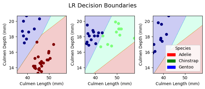
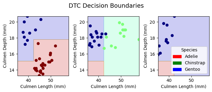

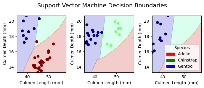
Conclusion
Through different machine learning algorithms that ouputed the same results, we selected culmen length, culmen depth, and thr island the penguins are from as the best features for classification. After our comparison between models, we found our best model to be the logistic regression model with both the training and testing accuracies of 100%. The second best models were the random forest and the decision tree models with a training accuracy of 100% and a test accuracy of 98.5%. The least effective model in our evaluation was the support vector machine, with a training accuracy of 98.0% and a test accuracy of 92.6%. Overall, the feature selection and the classification showed high accuracies and were considered successful. If we had time, we would include more columns from the original dataset to train for finding the best features. In that way, we could also see if our model performance would enhance.