from perceptron import Perceptronsource code link: https://github.com/yanruoz/yanruoz.github.io/blob/main/posts/perceptron/perceptron.py
Implementation of the Perceptron Update
In the fit() function, I first reset history as an empty array to avoid accumulating histories of multiple datasets. Then, I unpack the tuple returned by X.shape by assigning the number of data points to n, and the number of features to p. Then, I initialize a random initial weight vector w_tilt(0) as a 1D array composed of floats \(\in [1, -1]\). Next, I modify the input X into X_ (which contains a column of 1s and corresponds to X_tilde).
Within the for loop that iterates within the range of the max steps input by the user, I generate a random number within the amount of data points (n). We have the equation for the perceptron update: \(\tilde{w}^{(t+1)}=\tilde{w}^{(t)}+ \mathbb{1}{(\tilde{y_i} \langle \tilde{w}^{(t)}, \tilde{x_i} \rangle <0)}\tilde{y_i} \tilde{x_i}\), where \(\tilde{y_i} = 2y_i-1\) to make \(\tilde{y_i}\) take the value of (-1 and 1) instead of (0 and 1). To implement it, I calculate different parts of the equation respectively and update the weight by multiplying them:
---
y_tilde_i = 2 * y[i] - 1
x_tilde_i = X_[i]
y_tilde_pred = int(y_tilde_i * np.dot(x_tilde_i, self.w) < 0)
self.w += y_tilde_pred * y_tilde_i * x_tilde_i
---%load_ext autoreload
%autoreload 2import numpy as np
import pandas as pd
import seaborn as sns
from matplotlib import pyplot as plt
import random
from sklearn.datasets import make_blobs
from sklearn.datasets import make_moonsExperiment
Experiment 1: Linearly-separable 2d data
Using a 2d dataset in which the data is linearly separable, the perceptron algorithm converges to weight vector \(\tilde{w}\), which is the separating line shown in Fig 1.1.
np.random.seed(12345)

n = 100
p_features = 3

X, y = make_blobs(n_samples = n, n_features = p_features - 1, centers = [(-1.7, -1.7), (1.7, 1.7)])
fig = plt.scatter(X[:,0], X[:,1], c = y)
plt.title("Fig 1.1: Linearly separable 2d data points")
xlab = plt.xlabel("Feature 1")
ylab = plt.ylabel("Feature 2")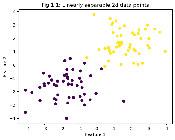
The evolution of the accuracy over training is shown in the printed history and Fig 1.2; the final accuracy of 1 confirms that the perceptron algorithm converges.
np.random.seed(12345)
p = Perceptron()
p.fit(X, y, max_steps = 10000)
p.w
print(p.history[-10:])
fig = plt.plot(p.history)
plt.title("Fig 1.2: Evolution of the accuracy over training of linearly separable 2d data")
xlab = plt.xlabel("Iteration")
ylab = plt.ylabel("Accuracy")
[0.99, 0.99, 0.99, 0.99, 0.99, 0.99, 0.99, 0.99, 0.99, 1.0]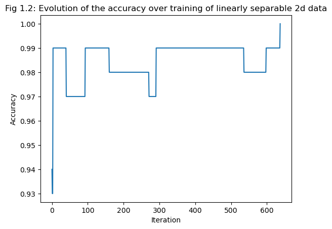
np.random.seed(12345)
def draw_line(w, x_min, x_max):
  x = np.linspace(x_min, x_max, 101)
  y = -(w[0]*x + w[2])/w[1]
  plt.plot(x, y, color = "black")

fig = plt.scatter(X[:,0], X[:,1], c = y)
fig = draw_line(p.w, -2, 2)
plt.title("Fig 1.3: Linearly separable 2d data points with the separating line")
xlab = plt.xlabel("Feature 1")
ylab = plt.ylabel("Feature 2")

p.score(X, y)
1.0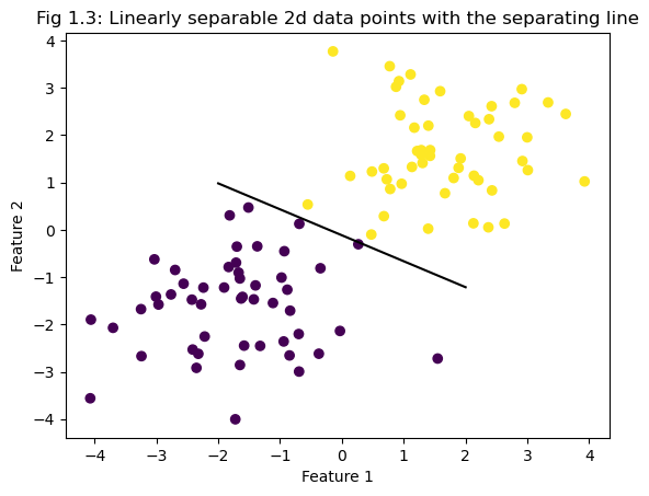
Experiment 2: Non-linearly-separable 2d data
In the case of not linearly separable 2d data, we generate such a dataset using make_moons function. As shown in the Fig 2.1, the data overlaps in a way that is not linearly separable.
np.random.seed(123)
# Generate a non-linearly separable dataset with 100 samples
X, y = make_moons(n_samples=100, noise=0.1, random_state=42)

# Plot the dataset
plt.scatter(X[:, 0], X[:, 1], c=y, cmap=plt.cm.Paired)
plt.title("Fig 2.1: Non-linearly-separable 2d data points")
plt.show()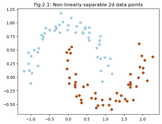
The evolution of accuracy over training also shows that the algorithm does not converge when the iteration of max steps is completed.
np.random.seed(123)
p = Perceptron()
p.fit(X, y, max_steps = 1000)
p.w
print(p.history[-10:])
fig = plt.plot(p.history)
xlab = plt.xlabel("Iteration")
ylab = plt.ylabel("Accuracy")
[0.86, 0.86, 0.86, 0.86, 0.86, 0.86, 0.86, 0.86, 0.86, 0.86]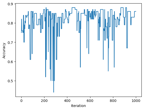
The separating line in the final iteration is shown in Fig.2.3, which does not separate the data obviously.
np.random.seed(123)
def draw_line(w, x_min, x_max):
  x = np.linspace(x_min, x_max, 101)
  y = -(w[0]*x + w[2])/w[1]
  plt.plot(x, y, color = "black")

fig = plt.scatter(X[:,0], X[:,1], c = y)
fig = draw_line(p.w, -2, 2)
plt.title("Fig 2.3: Non-linearly-separable 2d data points with the separating line")
xlab = plt.xlabel("Feature 1")
ylab = plt.ylabel("Feature 2")

p.score(X, y)
0.86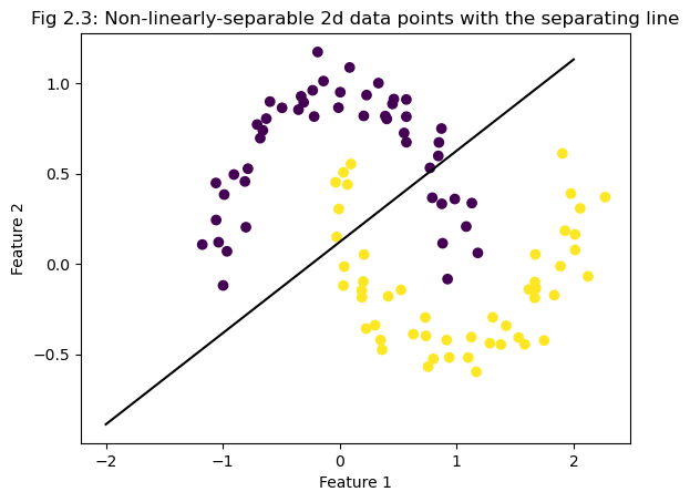
Experiment 3: 5d data
The perceptron algorithm is also able to work in more than 2 dimensions. In this experiment, the dataset has 5 features. The evolution of the accuracy over training is shown in Fig 3. Since the final score is less than 1, the algorithm does not converge; therefore, the data is not linearly separable.
np.random.seed(230230)

n = 100
p_features = 5

X, y = make_blobs(n_samples = n, n_features = p_features - 1, centers = [(-1.7, -1.7), (1.7, 1.7)])

p = Perceptron()
p.fit(X, y, max_steps = 1000)
p.w
print(p.history[-10:])
fig = plt.plot(p.history)
plt.title("Fig 1.2: Evolution of the accuracy over training of 5d data")
xlab = plt.xlabel("Iteration")
ylab = plt.ylabel("Accuracy")
[0.99, 0.98, 0.98, 0.98, 0.98, 0.98, 0.98, 0.98, 0.98, 0.98]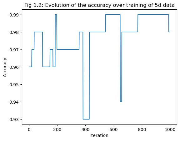
Thinking Question
Q: What is the runtime complexity of a single iteration of the perceptron algorithm update as described by Equation 1? Assume that the relevant operations are addition and multiplication. Does the runtime complexity depend on the number of data points ? What about the number of features?
R: The runtime complexity of a single iteration is \(O(N)\) because when calculating the dot product between the weight and the feature vector, we only consider one data point at a time. Therefore, the runtime complexity only depends on the number of features and not on the number of data points in a single iteration.